Non-Contact Measurement vs. Flow Velocity: A Selection Guide for Smart Water Management Scenarios

Introduction: From Single Readings to a Flow Evidence Chain

As urban drainage and flood control, irrigation-district metering, river monitoring, and industrial wastewater treatment place higher demands on flow data, Doppler flow meters are evolving from standalone velocity-measurement devices into flow-sensing systems coordinated with water level, cross-section, non-contact measurement, and integrated cameras.

In the past, project owners often asked, “Which device has higher accuracy?” Today, the more common question is: under sediment-laden, aerated, partially full, flood-season high-water-level, or low-illumination nighttime conditions, how can verifiable velocity, water level, and flow results be obtained continuously?

Industry observations show that flow-metering errors often arise not only from the sensor itself but also from installation location, cross-section geometry, medium condition, operation and maintenance including dredging and cleaning, and data-fusion algorithms.

This article compares contact Doppler ultrasonic, radar non-contact measurement, pressure-type water-level fusion, and integrated-camera visual flow measurement technologies, and provides parameters, case studies, and selection recommendations for drainage pipe networks, open channels, rivers, and industrial discharge outlets.

Technology Route Overview: Same Objective, Different Physical Paths

Common flow-measurement technology routes can be grouped into four categories:

• Contact Doppler Ultrasonic Flow Meter: Measures point velocity from Doppler frequency shifts of echoes scattered by bodies in the acoustic beam. Suitable for liquids containing bubbles, suspended particles, or impurities.
• Radar or Microwave Non-Contact Measurement: Emits electromagnetic waves toward the water surface and obtains surface velocity from Doppler shift or phase difference. Often combined with level gauges and cross-section models.
• Pressure-Type or Ultrasonic Level Gauges: Fused with cross-section hydraulic models to infer flow area and flow rate from water level.
• Integrated-Camera Visual Flow Measurement: Uses image texture, floating particles, or artificial markers to estimate velocity while providing image evidence.

Doppler Ultrasonic Flow Meter: A Mature Route for Fluids Containing Impurities

The core of a Doppler ultrasonic flow meter is the frequency shift produced when an acoustic beam encounters scatterers such as bubbles, sediment, or flocs in water. The device typically emits ultrasound at 20 kHz to 60 kHz, receives echoes, and calculates the velocity component along the acoustic beam.

If installation angle, speed-of-sound compensation, and temperature compensation are correct, it can provide fast velocity response in full-pipe or open-channel conditions, making it suitable for wastewater treatment plant influent, industrial wastewater, rainwater discharge outlets, and drainage pipes.

Boundary Conditions & Challenges

• Medium Dependence: If water is too clear (scatterers insufficient), echo signal-to-noise ratio decreases. At a river cross-section, when sediment fell below 30 mg/L, velocity drift exceeded 15%.
• Bubbles and Grease: High gas content attenuates signals; surface grease contaminates transducers.
• Installation Coupling: Gaps between transducer and pipe wall amplify acoustic-path errors.
• O&M Drift: Probe coverage by sludge/biofilm causes gradual data drift.

Radar and Microwave Non-Contact Measurement: From Surface Velocity to Cross-Section Flow

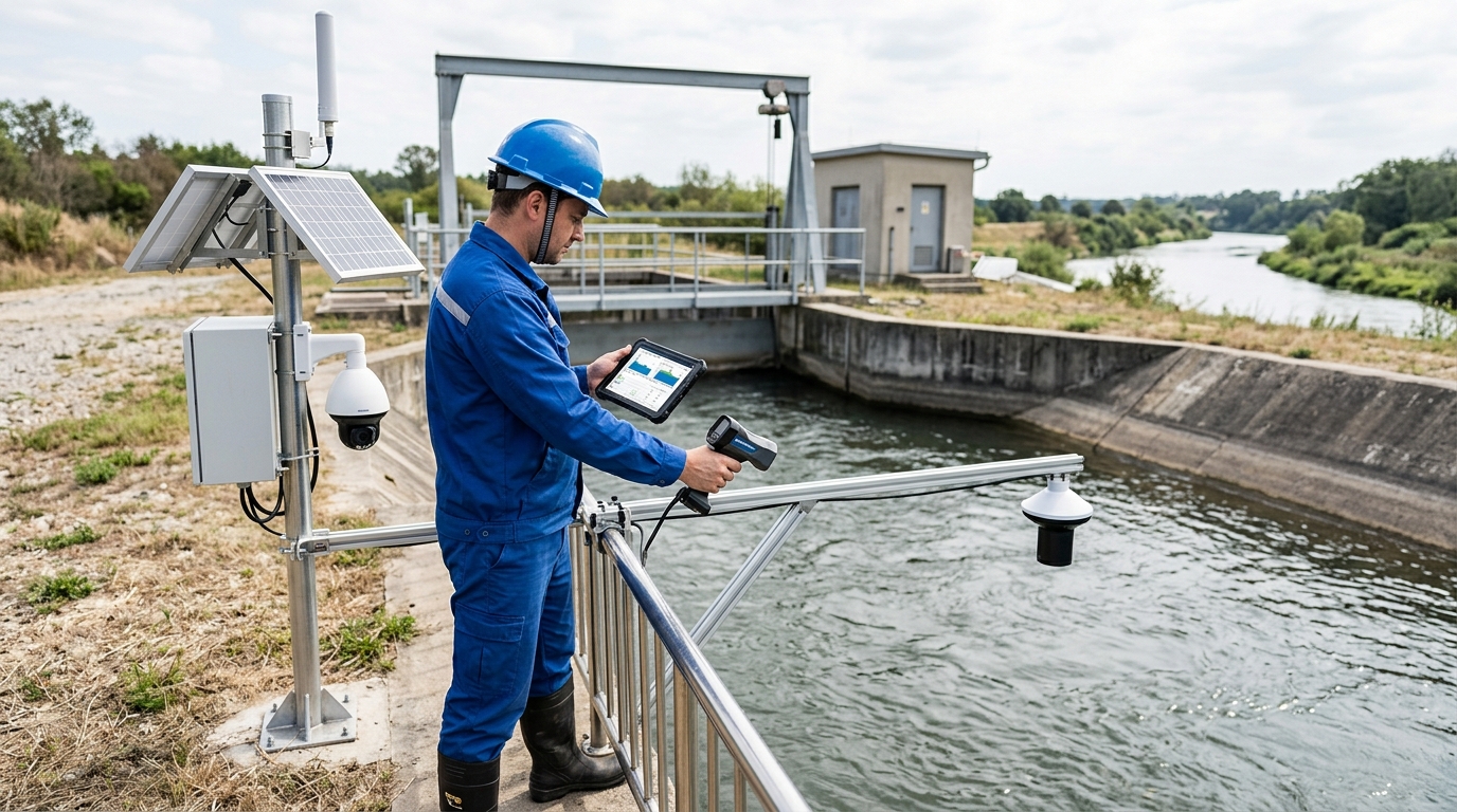
Radar and microwave technologies are typical non-contact measurement routes. Devices are installed at pipe tops, bridges, or poles, emitting electromagnetic waves toward the water surface. Because the sensor does not contact the medium, it avoids probe fouling issues, offering clear O&M advantages in wastewater and river applications.

Common installation heights are 1 m to 10 m (up to 30 m for some devices). For open channels and rivers, radar velocity meters are usually paired with pressure/ultrasonic level gauges and cross-section libraries to convert surface velocity into cross-section average velocity.

Cross-Section Calculation Logic

Radar rarely operates alone. It provides surface velocity; water level gauge provides depth; cross-section library provides area; algorithm applies correction coefficient (typically 0.85–0.95 for channels, lower for wide shallow rivers). Ignoring correction may overestimate flow by 10–20%.

A river monitoring station using Radar + Pressure Level + Integrated Camera achieved ~97% online rate and ~4.3% relative deviation vs. hydrological station manual measurements during flood season.

Pressure-Type Water Level and Velocity Fusion: A Key Variable in Shallow-Water Conditions

The pressure-type water level gauge is the “foundation” of many flow solutions. It converts static pressure to water level (Range 0–10m, Accuracy ±0.1%FS). In drainage networks and rivers, water level directly determines flow area and sets installation reference for other sensors.

For partially full pipes, when depth is only 0.3 m to 0.8 m, a ±2 cm water-level error may cause a ±6% to ±10% flow error. Water-level accuracy is a key variable determining flow result credibility.

Integrated Cameras and Visual Flow Measurement: From Numerical Output to Traceable Evidence

Integrated cameras add a new dimension: recording water-surface condition, debris, color anomalies, overflow traces, and personnel operations. Typical config: 2–5 MP industrial camera, 30–60 fps, supplemental lighting/polarizers, aligned with radar/water level angles.

Visual algorithms extract motion from texture/foam/particles. Under stable lighting/features, velocity accuracy is ±5%–±10%. Best suited for auxiliary verification and evidence preservation rather than sole metering basis.

Limitations: Nighttime, heavy rain, fog, snow, and strong backlighting reduce image quality. Low illumination increases texture extraction failure rates unless supplemental lighting is sufficient.

Selection Recommendations: Decide Based on Medium, Operating Conditions, Accuracy, and Operation and Maintenance

Cost & O&M Decision Variables

Avoid comparing only unit prices. Calculate comprehensive cost of 3-year O&M, comparative testing, downtime, and data disputes.

• Doppler: Lower initial investment, but frequent probe cleaning/coupling checks (1–2 inspections/month in sewers).
• Radar: Higher initial investment, but non-contact = less dredging, suitable for unattended long-term operation.
• Pressure Level: Low cost, but requires periodic calibration for blockage/zero drift.
• Cameras: Increases hardware/storage/transmission/algorithm costs, but improves data credibility and traceability.

For critical nodes with ±5% accuracy target, redundant configuration of velocity, water level, and imagery is recommended.

Outlook: Toward Integrated “Sensing–Algorithm–Evidence Chain” Systems

Future flow monitoring moves from “measuring one number” to integrated systems. Devices will increasingly combine Doppler, radar, pressure level, temperature, orientation, and camera modules with edge computing for real-time data quality assessment.

Example: System detects installation-angle offset, surface foam, or zero drift → automatically reduces confidence, triggers cleaning, or notifies inspection. Algorithms will fuse velocity, water level, and imagery using cross-section libraries, hydrodynamic models, and AI recognition to improve stability in complex conditions.

Technical competitiveness expands from single-transducer performance to system coordination capability. Future acceptance emphasizes continuous online rate, abnormal event traceability, fusion deviation, and image evidence completeness.

Industry standardization affects selection. Flow metering involves installation, comparative testing, correction coefficients, data retention, and fault handling—not just sensor accuracy. Choosing a route is finding balance among these factors.